Seasonal Decomposition of MRR

Overview

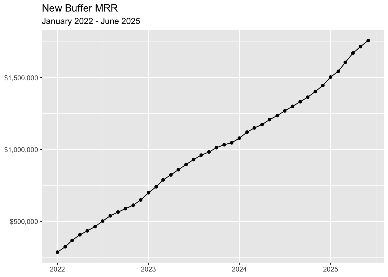
In this analysis we’ll analyze Buffer’s MRR data and break it down into its seasonal components. We’ll do a seasonal decomposition to isolate the trend, seasonal component, and residual.

The data we’ll use comes from ChartMogul, but you can view our transparent revenue data for yourself here.

Code

# read csv from Mixpanel
mrr <- read.csv("~/Downloads/mrr.csv")

# set date as date
mrr <- mrr %>% 
  mutate(ymd = ymd(date),
         month = floor_date(ymd, unit = "months")) %>% 
  filter(month != max(month))

Seasonal Decomposition

It’s often helpful to break time series data down into its various components. For example, it’s useful to see if data tends to behave a certain way in a given month or on a given day of the week.

For our MRR time series data we’ll break it down into three distinct components:

Trend: a trend is present when there is a long-term increase or decrease in the data. In our case, we could probably use a simple linear regression model to extract the trend.
Seasonal: a seasonal pattern occurs when a time series is affected by seasonal factors such as the time of the year or the day of the week. In our case, since our data is monthly, we’ll look at the time of year.
Residual: everything else, after accounting for the trend and seasonal component.

For this analysis we’ll use SEATS decomposition. SEATS stands for Seasonal Extraction in ARIMA Time Series. This method was developed at the Bank of Spain and is now widely used by government agencies around the world.

Code

# convert data to time series object
mrr_ts <- ts(mrr$mrr, 
             start = c(2022, 1),  
             frequency = 12)

# plot seasonal decomposition
mrr_ts %>% 
  seas(x11 = "") %>%
  autoplot() +
  geom_point() +
  labs(x = "Month",
       title = "Seasonal Decomposition of New Buffer MRR Data") +
  scale_y_continuous(labels = dollar)

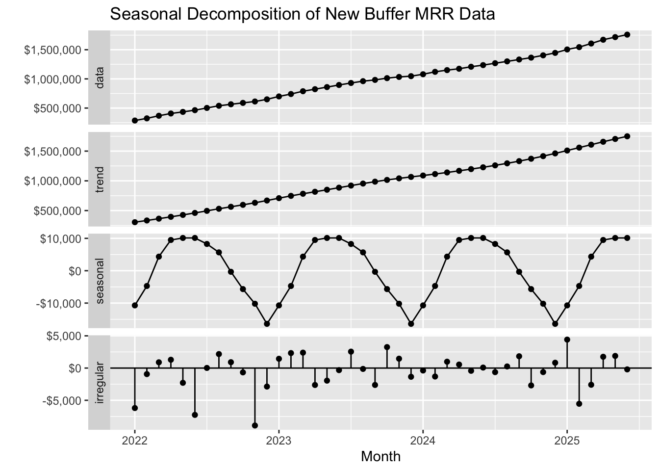
The plot above shows the the actual MRR data in the top plot, the trend below that, the seasonal component, and finally the residuals (what remains after adding the seasonal component to the trend).

The seasonal component suggests that MRR growth tends to be higher in the beginning of the year and slows towards the end of the year, starting in July.