This analysis follows a similar structure to previous analyses on posting frequency, but focuses specifically on TikTok. Like in those analyses, our goal is to explore how weekly posting frequency relates to post performance, with views as the primary engagement metric.
What We Found
When we compare channels to themselves over time, posting more frequently on TikTok is associated with more views per post. The results of a fixed‑effects regression model that accounts for account-level differences suggests that weeks with 2–5 posts see roughly 20% more views per post than weeks in which only one post was sent. Weeks with 6–10 posts yield about 36% more views per post, and weeks with 11+ posts yield about 44% more. Adding calendar‑week fixed effects yields slightly smaller but very similar effects (about 17%, 29%, and 34%).
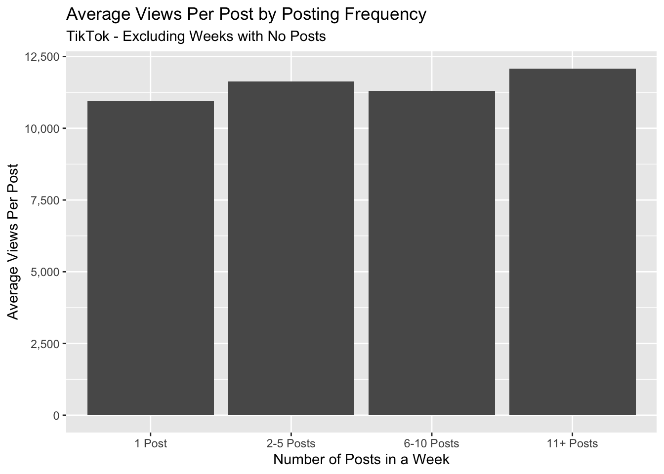
At the same time, the simple summary statistics (like averages and medians) paint a more nuanced picture. Average views per post are fairly flat across bins and the median falls a bit at higher cadences.
This implies that the distribution of views per post becomes more skewed at higher posting frequency, even if the typical post doesn’t necessarily perform better.
Given that, my takeaway would be that increasing posting frequency on TikTok does tend to lift the number of views per post, but not in a uniform way. For me, the more important thing is that posting more frequently does not necessarily lift the typical post, but it does increase the likelihood of having breakout posts that go viral.
The Z‑score analysis is also helpful here because it compares each channel to its own baseline and avoids cross‑account confounding. Summaries by posting‑frequency bin point in the same direction as the regression: relative performance improves as posting frequency increases, with the largest step occurring between one post and two to five posts per week.
If we wanted to provide a blanket recommendation that applies to most people, I’d recommend starting with 2-5 posts per week on TikTok. However, if you have more posts to share, you’ll give yourself a better chance at having a breakout post.
Methodology
This analysis examines how posting frequency affects view counts on TikTok. We’ll start by grouping posting frequency into bins (1 post, 2–5 posts, 6–10 posts, 11+ posts per week) and then analyze post performance within these bins.
We’ll then use Z-scores and fixed effects regression to control for account-level differences and compare each account’s performance to its own baseline over time.
Data Collection
The SQL below outlines the extraction of TikTok posts and views from dbt_buffer.publish_updates. We restrict the data to the past 365 days and only include profiles with enough activity.
Code
sql <-"with qualified_tiktok_profiles as ( -- profiles that posted in at least 4 weeks in the past year and have views select up.profile_id , count(distinct timestamp_trunc(up.sent_at, week)) as weeks_with_posts , sum(up.views) as total_views , count(distinct up.id) as total_posts from dbt_buffer.publish_updates as up where up.profile_service = 'tiktok' and up.sent_at >= timestamp_sub(current_timestamp, interval 365 day) and coalesce(up.views, 0) > 0 group by 1 having count(distinct timestamp_trunc(up.sent_at, week)) >= 4),posts_with_week_stats as ( select up.profile_id , timestamp_trunc(up.sent_at, week) as week , up.id , coalesce(up.views, 0) as views , coalesce(up.likes, 0) as likes , coalesce(up.comments, 0) as comments , coalesce(up.shares, 0) as shares , coalesce(up.reach, null) as reach , up.media_type , percentile_cont(coalesce(up.views, 0), 0.5) over (partition by up.profile_id, timestamp_trunc(up.sent_at, week)) as median_views from dbt_buffer.publish_updates as up inner join qualified_tiktok_profiles as qtp on up.profile_id = qtp.profile_id where up.profile_service = 'tiktok' and up.sent_at >= timestamp_sub(current_timestamp, interval 365 day))select profile_id as channel_id , week , count(distinct id) as posts , sum(views) as total_views , sum(likes) as total_likes , sum(comments) as total_comments , sum(shares) as total_shares , avg(nullif(views, 0)) as avg_views , max(median_views) as median_viewsfrom posts_with_week_statsgroup by 1, 2order by 1, 2"# get data from BigQueryposts <-bq_query(sql = sql)
This query returns around 11.4 million posts from 151 thousand TikTok profiles.
We’ll group the number of posts sent in a given week into frequency buckets similar to previous analyses.
Our primary will be on the number of views per post. This should more accurately measure the efficiency of posting strategies rather than the effect of more volume.
Here are some summary statistics for each posting frequency bin:
Code
# per-post and log-scale summaries by frequency binengagement_per_post %>%group_by(posting_frequency_bin) %>%summarise(n_observations =n(),avg_views_per_post =mean(views_per_post, na.rm =TRUE),median_views_per_post =median(views_per_post, na.rm =TRUE),avg_log_views_per_post =mean(log_views_per_post, na.rm =TRUE) )
# plot average views per post by posting frequency (raw scale)engagement_per_post %>%group_by(posting_frequency_bin) %>%summarise(avg_views_per_post =sum(total_views) /sum(posts)) %>%ggplot(aes(x = posting_frequency_bin, y = avg_views_per_post)) +geom_col(show.legend =FALSE) +scale_y_continuous(labels = comma) +labs(x ="Number of Posts in a Week",y ="Average Views Per Post",title ="Average Views Per Post by Posting Frequency",subtitle ="TikTok - Excluding Weeks with No Posts")
Because there is a huge amount of variance in the number of views that posts get, applying a log transformation is useful here. Taking logs stabilizes variance and reduces the influence of occasional breakout posts, making comparisons across posting‑frequency bins more representative of typical performance.
Code
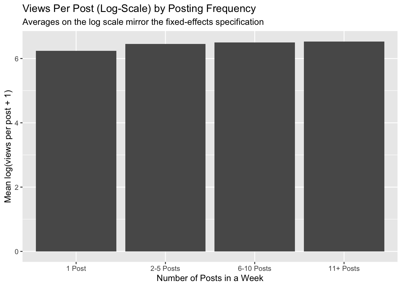
# plot log-scale mean to align with FE modelengagement_per_post %>%group_by(posting_frequency_bin) %>%summarise(avg_log_views =mean(log_views_per_post, na.rm =TRUE)) %>%ggplot(aes(x = posting_frequency_bin, y = avg_log_views)) +geom_col(show.legend =FALSE) +labs(x ="Number of Posts in a Week",y ="Mean log(views per post + 1)",title ="Views Per Post (Log-Scale) by Posting Frequency",subtitle ="Averages on the log scale mirror the fixed-effects specification")
On the log scale, average views per post tend to rise steadily with posting frequency. Moving from 1 post to 2–5 posts corresponds to about a 25% lift in views per post on average; 6–10 posts is roughly 30% higher than one post, and 11+ posts is about 34% higher.
The step-up from 1 to 2–5 posts is the biggest, with smaller gains at higher cadences, which suggests diminishing returns. That being said, this is still a basic summary statistic, and we’ll want to use a more robust approach to control for differences between accounts.
Statistical Challenges and Our Approach
These summary statistics show interesting patterns, but they may not tell us the full story. As in our previous analyses, we still need to control for differences in accounts’ inherent differences, such as the number of followers.
To illustrate the need for controlling these factors, imagine a high-engagement account that naturally gets a lot of views and tends to post frequently, versus a smaller account that gets less views and posts less often. If we simply compare across accounts, we might incorrectly conclude that posting frequency drives more views per post, when in reality it could be that high-performing accounts simply tend to post more.
To address this issue, we use statistical methods that compare each account against itself over time, basically asking the question “when this account posts more or less frequently, how does their view counts change?” This within-account comparison controls for inherent differences between accounts.
How We Account for Inherent Account Differences
We use two complementary approaches to ensure that we’re measuring the true effect of posting frequency:
Z-score analysis: Instead of comparing different channels to each other, we compare each profile to its overall average number of views per post. The Z-score tells us how much better or worse a profile performed compared to its own average.
For example, if Channel A typically gets 500 views per post and Channel B typically gets 100 views per post, a week with 300 views per post would be below average for Channel A, represented by a negative Z-score, and above average for Channel B, represented by a positive Z-score.
Fixed effects regression: This statistical technique controls for all time-invariant account characteristics. It attempts to answer the question “when the same channel varies its posting frequency across different weeks, how does this affect their per-post performance?”
This method compares each channel’s high-frequency weeks to their own low-frequency weeks, controlling for the inherent differences between accounts that remain constant over time.
Z-Score Analysis
Let’s start by calculating Z-scores for each channel. We’ll apply a log transformation for the reasons stated earlier.
Code
# Z-score computation on log(views per post + 1)channel_stats_per_post <- engagement_per_post %>%group_by(channel_id) %>%summarise(mean_log_views_per_post =mean(log_views_per_post, na.rm =TRUE),sd_log_views_per_post =sd(log_views_per_post, na.rm =TRUE),n_weeks =n() ) %>%filter(n_weeks >=3, sd_log_views_per_post >0)# calculate Z-scores on log scaleengagement_per_post_with_z <- engagement_per_post %>%inner_join(channel_stats_per_post, by ="channel_id") %>%mutate(z_log_views_per_post = (log_views_per_post - mean_log_views_per_post) / sd_log_views_per_post)# average Z-scores by posting frequency bin (mean)zscore_summary <- engagement_per_post_with_z %>%group_by(posting_frequency_bin) %>%summarise(mean_z_log_views_per_post =mean(z_log_views_per_post, na.rm =TRUE))zscore_summary
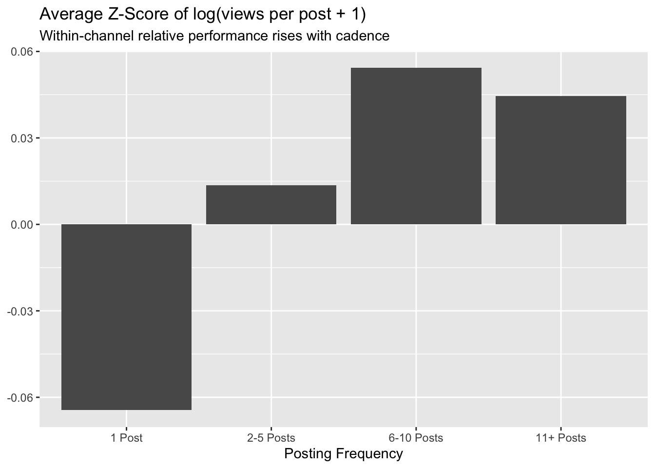
# Z-score plot (mean of log-scale Z-scores)zscore_summary %>%ggplot(aes(x = posting_frequency_bin, y = mean_z_log_views_per_post)) +geom_col(show.legend =FALSE) +labs(x ="Posting Frequency", y =NULL,title ="Average Z-Score of log(views per post + 1)",subtitle ="Within-channel relative performance rises with cadence")
On the log scale, average Z-scores increase with posting frequency. Relative to weeks with only one post, weeks with 2-5 posts show a small increase from each channel’s own baseline, with a further increase at 6-10 posts and a slight decrease at 11+.
The pattern is consistent with diminishing but still positive returns as posting frequency increases. The reasons why this might be are interesting to explore. We suspect that TikTok’s algorithm could reward more frequent posting, but there may also be other important factors at play, such as increased chances of hitting on a viral post.
This is why we want to understand how the upper end of the tail behaves as posting frequency increases. TikTok views are famously heavy‑tailed, meaning that most posts get modest numbers, while a small fraction take off.
Looking at the 90th percentile (“p90”) alongside the median lets us separate typical performance (what most posts do) from breakout potential (what strong posts can do). If p90 grows faster than the median as cadence increases, it suggests posting more creates more opportunities for big hits, even if the typical post doesn’t change as much.
Here’s one way to think about it using our data. At one post per week, the median views per post is about 489 and the 90th percentile is about 3,722. That means a typical post gets around 500 views, and only about one in ten posts gets more than 3.7k views.
At 11+ posts per week, the median is still roughly the same (around 459), but the 90th percentile jumps to 14.4k. In other words, the “typical” post hasn’t improved meaningfully, but there are more opportunities for a post to take off, and the bar for a top post is much higher. The p90 / median ratio (how much larger strong posts are than typical posts) is a simple way to quantify that gap. My interpretation is that a larger ratio signifies a heavier tail and more potential for a post to go viral.
Code
# Skew and breakout-post view: p90 vs median by frequency bintail_summary <- engagement_per_post %>%group_by(posting_frequency_bin) %>%summarise(median_views =median(views_per_post, na.rm =TRUE),p90_views =quantile(views_per_post, 0.90, na.rm =TRUE) ) %>%mutate(ratio_p90_to_median = p90_views / median_views)tail_summary
# Plot p90 views per post by frequencytail_summary %>%ggplot(aes(x = posting_frequency_bin, y = p90_views)) +geom_col(show.legend =FALSE) +scale_y_continuous(labels = comma) +labs(x ="Posting Frequency",y ="90th Percentile Views Per Post",title ="Heavier Tails at Higher Posting Frequencies",subtitle ="Higher frequency increases p90 (more opportunities for viral posts)")
Code
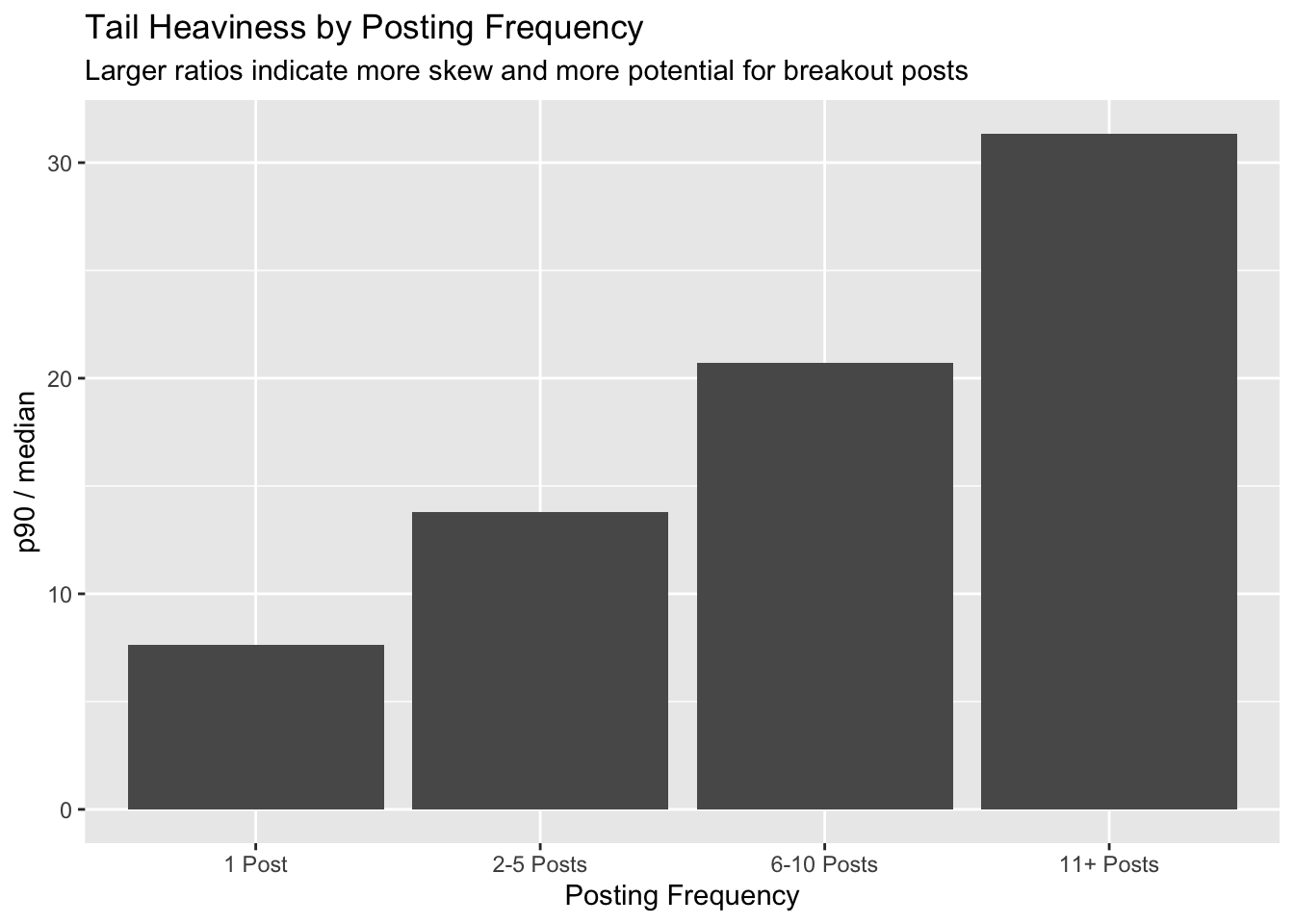
# Plot tail ratio directly: p90 / mediantail_summary %>%ggplot(aes(x = posting_frequency_bin, y = ratio_p90_to_median)) +geom_col(show.legend =FALSE) +labs(x ="Posting Frequency",y ="p90 / median",title ="Tail Heaviness by Posting Frequency",subtitle ="Larger ratios indicate more skew and more potential for breakout posts")
At the 90th percentile, views per post rise sharply with cadence: from roughly 3,700 at one post to about 7,000 at two to five posts, ~10,100 at six to ten, and ~14,400 at eleven or more. Meanwhile, medians are fairly flat to slightly lower (about 489 → 506 → 487 → 459), so the p90/median ratio jumps from ~7.6 to ~13.8 to ~20.7 to ~31.4.
The main takeaway here is that posting more frequently does not necessarily lift the typical post, but it does increase the likelihood of having a viral post that gets a lot of views.
Fixed Effects Regression Models for Per-Post Metrics
Fixed effects regression compares each profile to itself over time. Instead of asking whether accounts that post more get more views, which would mix together big and small accounts, we ask “when the same channel posts more in some weeks and less in others, how do its views per post change?”
This controls for all time‑invariant differences across channels. Things like audience size, niche, tone, or brand strength can be confounding factors. Effectively we’re measuring the change relative to each profile’s own baseline.
Because views are heavy‑tailed, we model views per post on a log scale. That helps in a couple of ways: it reduces the influence of the occasional viral week, and it makes the coefficients easy to read as approximate percent differences versus a one‑post week.
We also control for calendar week fixed effects, which account for platform‑wide shifts, such as algorithm changes, that affect everyone at the same time.
As a simple example, imagine a channel that typically posts once per week and averages 500 views per post. In weeks when that same channel posts five times, if its views per post are, say, 20% higher than its own baseline, the fixed effects model attributes that difference to posting frequency rather than to the channel simply being a larger account.
Code
# FE on log(views per post + 1), clustered by channelfe_log <-feols(log_views_per_post ~ posting_frequency_bin | channel_id, data = engagement_per_post, cluster ="channel_id")summary(fe_log)
Relative to weeks in which only one post was sent, posting 2–5 times per week is associated with around 20% higher views per post, on average, for the same channel. Posting 6–10 times results in 35% more views, on average, and 11+ posts is around 44% higher.
Code
# FE with calendar-week fixed effects in addition to channel FEfe_log_week <-feols(log_views_per_post ~ posting_frequency_bin | channel_id + week, data = engagement_per_post, cluster ="channel_id")summary(fe_log_week)
With calendar‑week fixed effects, the pattern is the same but the magnitudes are slightly smaller: 2–5 posts ≈ exp(0.160)−1 ≈ 17%, 6–10 posts ≈ exp(0.256)−1 ≈ 29%, and 11+ posts ≈ exp(0.294)−1 ≈ 34%. Accounting for platform‑wide shifts doesn’t change the conclusion: higher cadence is associated with higher per‑post views within the same channel, with diminishing returns at the very highest frequencies.
We should remember that this is likely due to the higher likelihood of a post going viral, rather than a steady increase in typical post performance.
Caveats and Limitations
As with any observational study, residual confounding remains possible. Views can be influenced by promotion, boosted distribution, or content trends that may correlate with frequency. Measurement on TikTok can also vary by format and counting windows. We’ve focused on the past year. Results could shift under a different time horizon or with alternative qualification thresholds.